4  Rozkłady i obserwacje odstające

Rozkłady odpowiadają na pytania: jakie wartości są typowe, jak szeroki jest zakres i czy dane mają ogon lub obserwacje odstające. To zwykle najlepszy punkt startu, zanim zaczniemy porównywać grupy.

library(tidyverse)
library(here)
library(janitor)
library(patchwork)

source(here("R", "theme_course.R"))
theme_set(theme_course())

fmr <- readr::read_csv(here("datasets", "FY18_4050_FMRs.csv"), show_col_types = FALSE) |>
  janitor::clean_names()

melb <- readr::read_csv(here("datasets", "melb_clean.csv"), show_col_types = FALSE) |>
  janitor::clean_names() |>
  select(-any_of("x1")) |>
  mutate(
    price_m = price / 1000000,
    region = recode(
      region,
      Northern = "Północny",
      Western = "Zachodni",
      Southern = "Południowy",
      Eastern = "Wschodni",
      `South-Eastern` = "Południowo-wschodni",
      `Eastern Victoria` = "Wschodnia Wiktoria",
      `Northern Victoria` = "Północna Wiktoria",
      `Western Victoria` = "Zachodnia Wiktoria"
    ),
    type = recode(type, h = "dom", u = "mieszkanie", t = "szeregowiec")
  )

school_grants <- readr::read_csv(
  here("datasets", "schoolimprovement2010grants.csv"),
  show_col_types = FALSE
) |>
  janitor::clean_names() |>
  select(-any_of("x1")) |>
  filter(!is.na(award_amount)) |>
  mutate(
    award_amount_m = award_amount / 1000000,
    model_selected = factor(
      recode(
        model_selected,
        Closure = "Zamknięcie",
        Restart = "Restart",
        Turnaround = "Restrukturyzacja",
        Transformation = "Transformacja"
      ),
      levels = c("Zamknięcie", "Restart", "Restrukturyzacja", "Transformacja")
    )
  )

bike_share <- readr::read_csv(
  here("datasets", "bike_share.csv"),
  show_col_types = FALSE
)

4.1 Histogram i wykres gęstości (density plot)

fmr |>
  ggplot(aes(x = fmr_2)) +
  geom_histogram(aes(y = after_stat(density)), bins = 35, fill = "#56B4E9", color = "white") +
  geom_density(colour = "#D55E00", linewidth = 1) +
  scale_x_continuous(labels = scales::label_dollar()) +
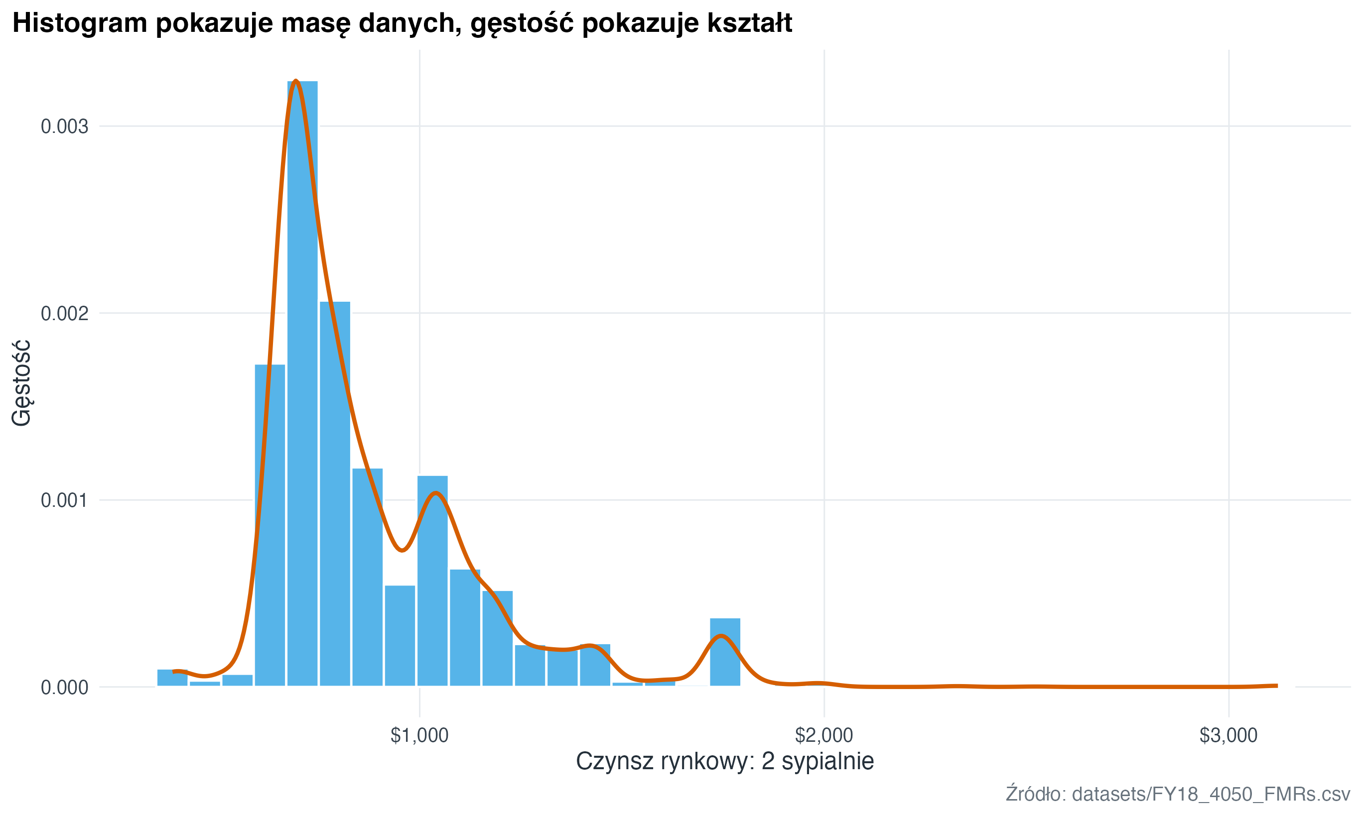
  labs(
    title = "Histogram pokazuje masę danych, gęstość pokazuje kształt",
    x = "Czynsz rynkowy: 2 sypialnie",
    y = "Gęstość",
    caption = "Źródło: datasets/FY18_4050_FMRs.csv"
  )

Rysunek 4.1: Rozkład czynszu rynkowego dla mieszkań z dwiema sypialniami.

4.2 Histogram, gęstość i kreski obserwacji (rug plot)

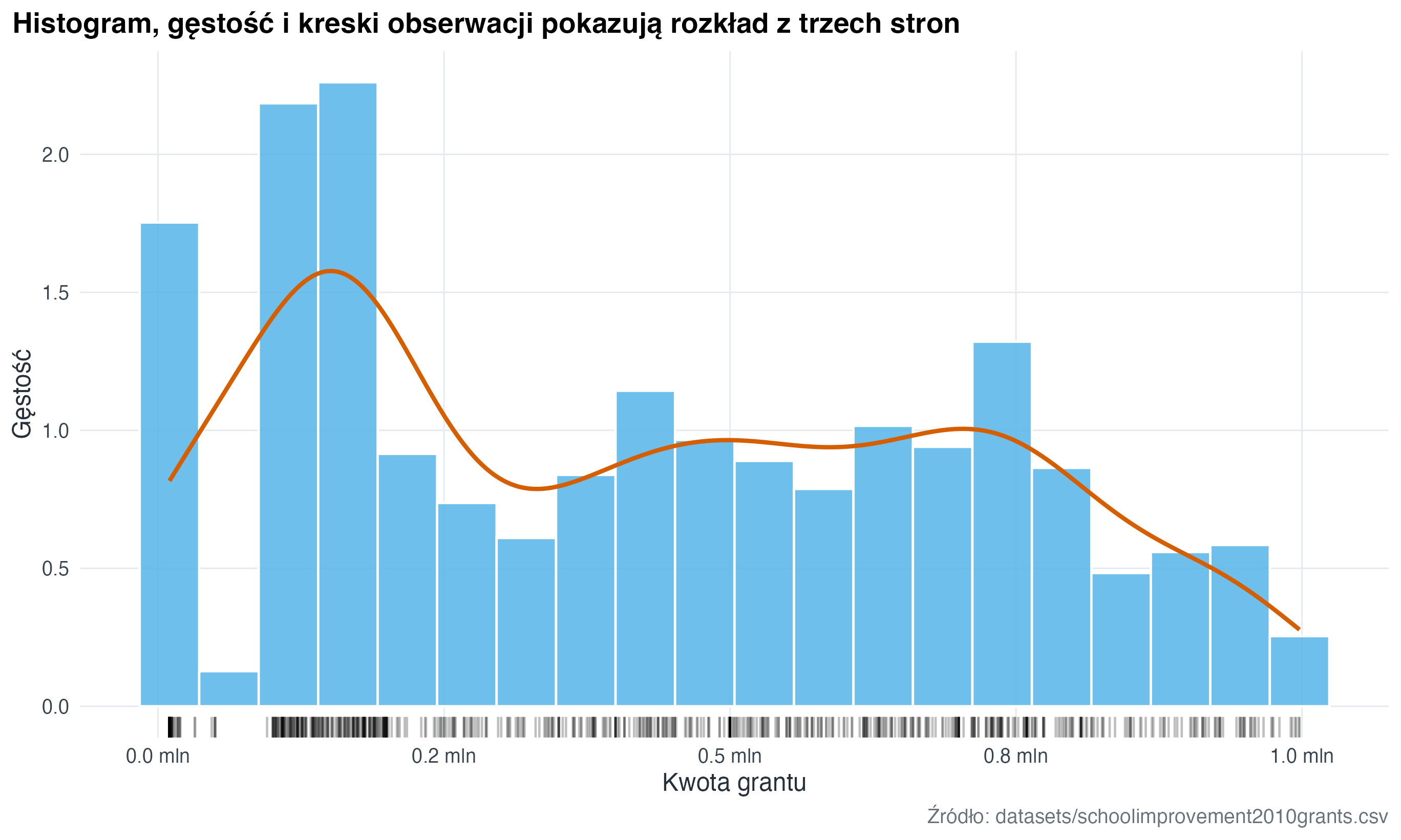
W R ten widok składamy jawnie z kilku warstw: histogramu, wykresu gęstości (density plot) i krótkich kresek pokazujących pojedyncze obserwacje (rug plot). Każda warstwa odpowiada na trochę inne pytanie o rozkład.

school_grants |>
  ggplot(aes(x = award_amount_m)) +
  geom_histogram(
    aes(y = after_stat(density)),
    bins = 20,
    fill = "#56B4E9",
    colour = "white",
    alpha = 0.86
  ) +
  geom_density(colour = "#D55E00", linewidth = 1) +
  geom_rug(alpha = 0.25, sides = "b") +
  scale_x_continuous(labels = scales::label_number(suffix = " mln", accuracy = 0.1)) +
  labs(
    title = "Histogram, gęstość i kreski obserwacji pokazują rozkład z trzech stron",
    x = "Kwota grantu",
    y = "Gęstość",
    caption = "Źródło: datasets/schoolimprovement2010grants.csv"
  )

Rysunek 4.2: Histogram grantów szkolnych z krzywą gęstości i kreskami obserwacji.

fmr_one_bed <- fmr |>
  filter(!is.na(fmr_1), dplyr::between(fmr_1, 300, 1500))

fmr_one_bed_stats <- fmr_one_bed |>
  summarise(
    mean_rent = mean(fmr_1),
    median_rent = median(fmr_1)
  )

fmr_one_bed |>
  ggplot(aes(x = fmr_1)) +
  geom_rect(
    data = fmr_one_bed_stats,
    aes(
      xmin = pmin(mean_rent, median_rent),
      xmax = pmax(mean_rent, median_rent)
    ),
    ymin = 0,
    ymax = Inf,
    fill = "#F0E442",
    alpha = 0.28,
    inherit.aes = FALSE
  ) +
  geom_histogram(
    aes(y = after_stat(density)),
    bins = 30,
    fill = "#009E73",
    colour = "white",
    alpha = 0.76
  ) +
  geom_density(colour = "#0072B2", linewidth = 1) +
  geom_vline(
    data = fmr_one_bed_stats,
    aes(xintercept = median_rent, linetype = "Mediana"),
    colour = "#CC79A7",
    linewidth = 1
  ) +
  geom_vline(
    data = fmr_one_bed_stats,
    aes(xintercept = mean_rent, linetype = "Średnia"),
    colour = "#D55E00",
    linewidth = 1
  ) +
  scale_linetype_manual(values = c("Mediana" = "dashed", "Średnia" = "solid"), name = NULL) +
  scale_x_continuous(labels = scales::label_dollar()) +
  labs(
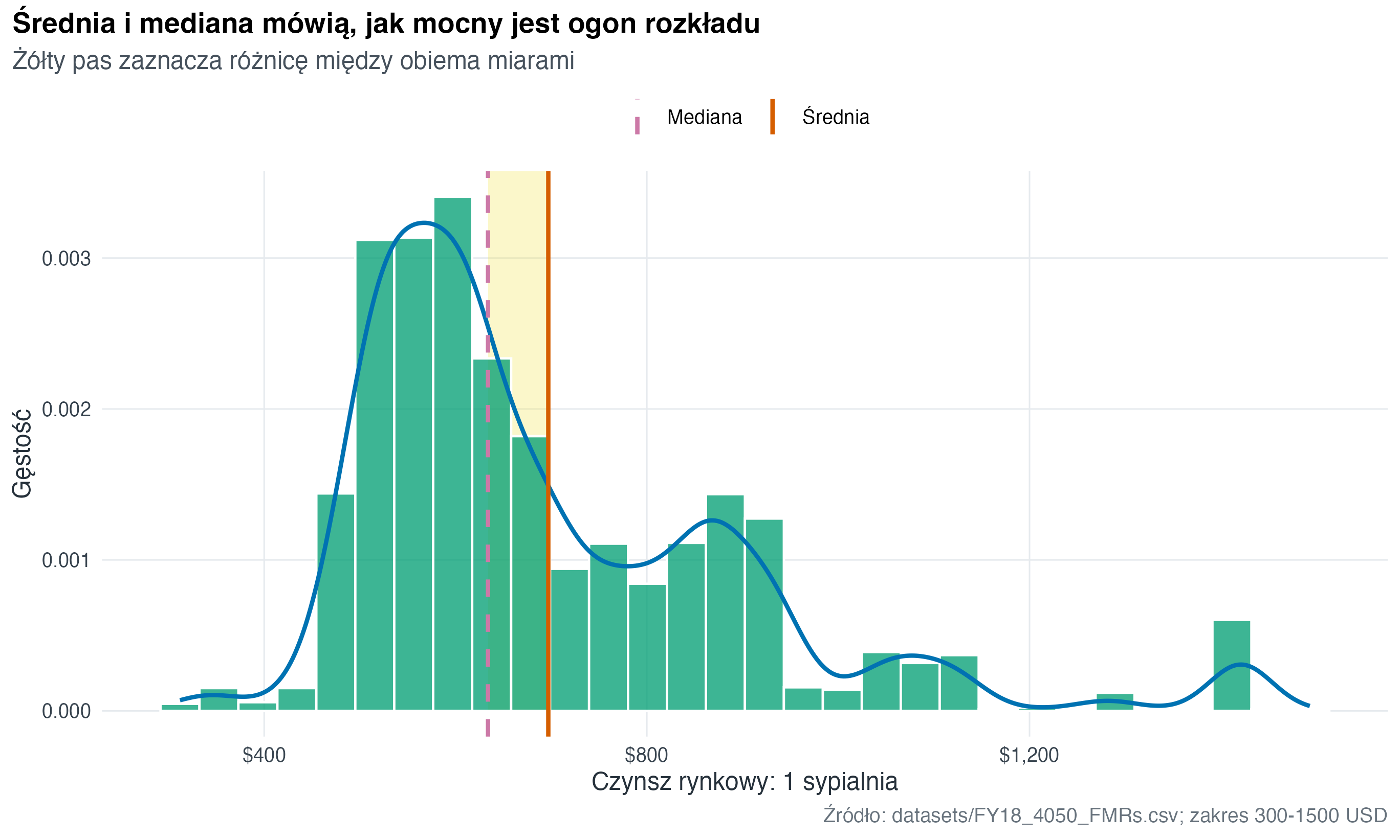
    title = "Średnia i mediana mówią, jak mocny jest ogon rozkładu",
    subtitle = "Żółty pas zaznacza różnicę między obiema miarami",
    x = "Czynsz rynkowy: 1 sypialnia",
    y = "Gęstość",
    caption = "Źródło: datasets/FY18_4050_FMRs.csv; zakres 300-1500 USD"
  )

Rysunek 4.3: Dopracowany histogram z medianą, średnią i zaznaczoną różnicą między nimi.

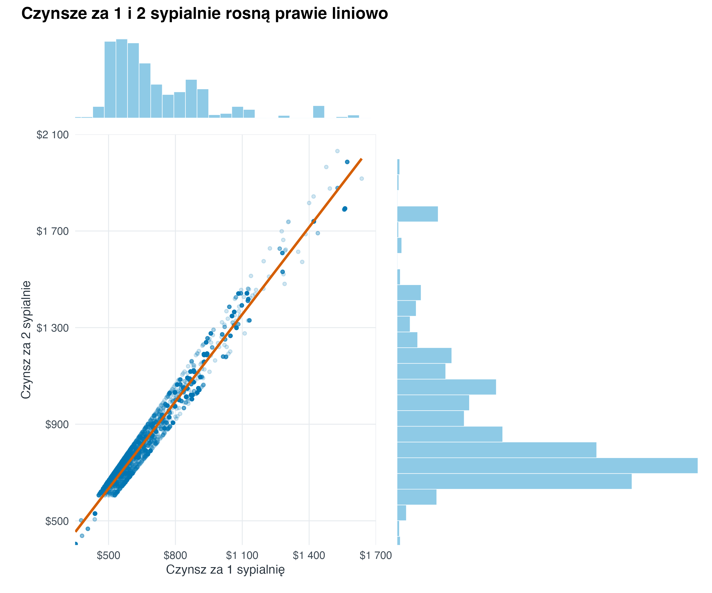
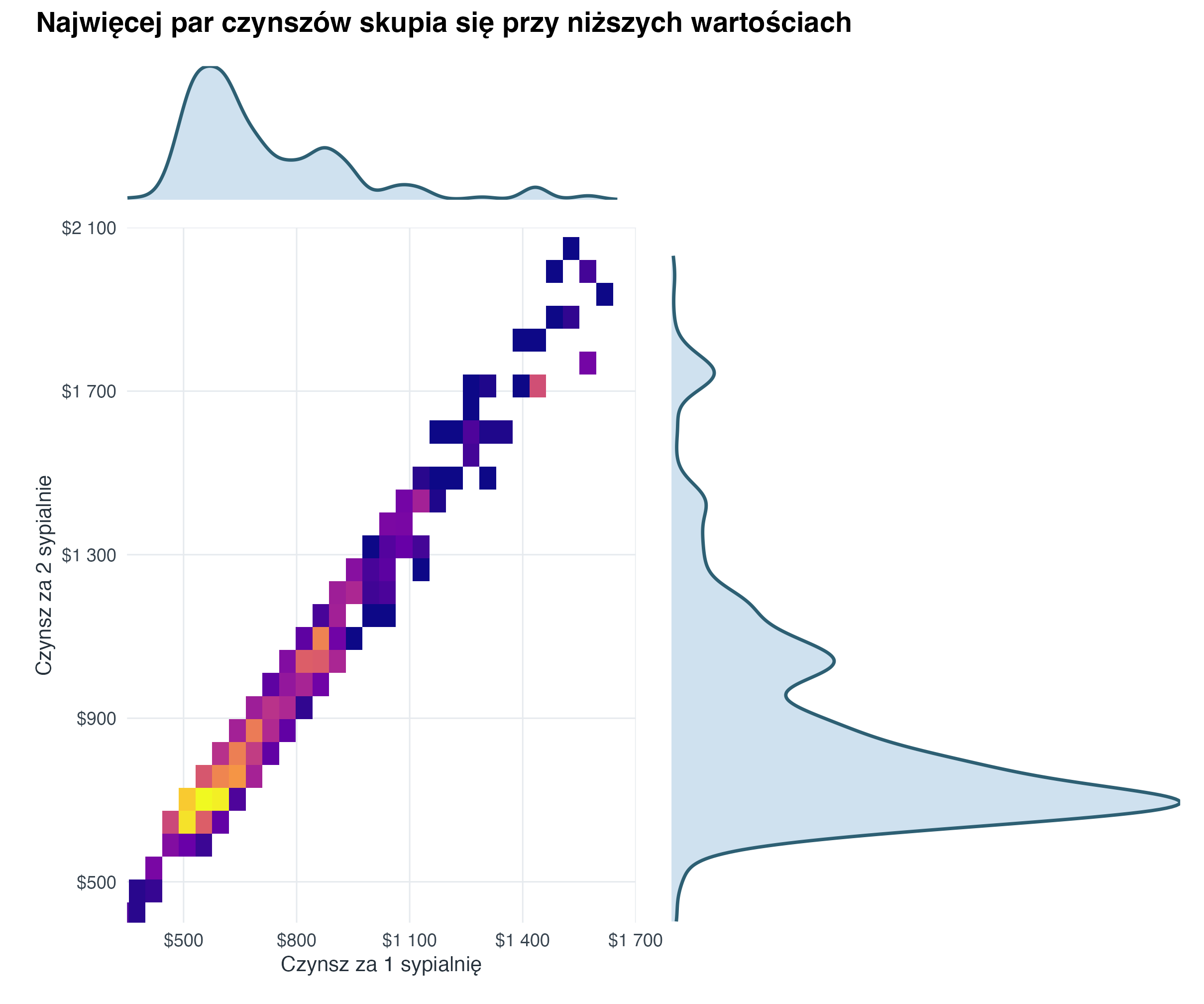
4.3 Wykres łączony: relacja i rozkłady brzegowe

Taki widok traktujemy jako kompozycję trzech elementów: głównego wykresu relacji oraz dwóch małych rozkładów brzegowych na osiach. Dzięki temu jednocześnie widać zależność między zmiennymi i kształt każdego rozkładu osobno.

fmr_joint <- fmr |>
  filter(
    !is.na(fmr_1),
    !is.na(fmr_2)
  )

rent_x_limits <- c(350, 1700)
rent_y_limits <- c(400, 2100)
rent_label <- scales::label_number(prefix = "$", big.mark = " ", accuracy = 1)

joint_plot_theme <- theme(
  axis.title = element_text(size = 10.5),
  axis.text = element_text(size = 9),
  plot.margin = margin(8, 12, 8, 12)
)

joint_margin_theme <- theme_void() +
  theme(plot.margin = margin(2, 6, 2, 6))

fmr_joint_visible <- fmr_joint |>
  filter(
    dplyr::between(fmr_1, rent_x_limits[1], rent_x_limits[2]),
    dplyr::between(fmr_2, rent_y_limits[1], rent_y_limits[2])
  )

joint_scatter <- fmr_joint_visible |>
  ggplot(aes(x = fmr_1, y = fmr_2)) +
  geom_point(alpha = 0.18, size = 1.1, colour = "#0072B2") +
  geom_smooth(method = "lm", se = FALSE, colour = "#D55E00", linewidth = 1) +
  coord_cartesian(xlim = rent_x_limits, ylim = rent_y_limits, expand = FALSE) +
  scale_x_continuous(
    labels = rent_label,
    breaks = seq(500, 1700, by = 300)
  ) +
  scale_y_continuous(
    labels = rent_label,
    breaks = seq(500, 2100, by = 400)
  ) +
  labs(
    x = "Czynsz za 1 sypialnię",
    y = "Czynsz za 2 sypialnie"
  ) +
  joint_plot_theme

joint_hist_x <- fmr_joint_visible |>
  ggplot(aes(x = fmr_1)) +
  geom_histogram(bins = 26, fill = "#8ECAE6", colour = "white", linewidth = 0.2) +
  coord_cartesian(xlim = rent_x_limits, expand = FALSE) +
  joint_margin_theme

joint_hist_y <- fmr_joint_visible |>
  ggplot(aes(x = fmr_2)) +
  geom_histogram(bins = 26, fill = "#8ECAE6", colour = "white", linewidth = 0.2) +
  coord_flip(xlim = rent_y_limits, expand = FALSE) +
  joint_margin_theme

((joint_hist_x + plot_spacer()) /
  (joint_scatter + joint_hist_y)) +
  plot_layout(widths = c(5.8, 1.15), heights = c(1, 5.2)) +
  plot_annotation(
    title = "Czynsze za 1 i 2 sypialnie rosną prawie liniowo",
    theme = theme(plot.title = element_text(face = "bold", size = 14, margin = margin(b = 8)))
  )

Rysunek 4.4: Wykres relacji z rozkładami brzegowymi: punkty, trend i histogramy marginalne. Skrajne wartości są przycięte dla czytelności.

joint_binned <- fmr_joint_visible |>
  ggplot(aes(x = fmr_1, y = fmr_2)) +
  geom_point(alpha = 0, size = 0, show.legend = FALSE) +
  geom_bin_2d(bins = 30, show.legend = FALSE) +
  coord_cartesian(xlim = rent_x_limits, ylim = rent_y_limits, expand = FALSE) +
  scale_fill_viridis_c(
    option = "C",
    trans = "sqrt"
  ) +
  scale_x_continuous(
    labels = rent_label,
    breaks = seq(500, 1700, by = 300)
  ) +
  scale_y_continuous(
    labels = rent_label,
    breaks = seq(500, 2100, by = 400)
  ) +
  labs(
    x = "Czynsz za 1 sypialnię",
    y = "Czynsz za 2 sypialnie"
  ) +
  joint_plot_theme

joint_density_x <- fmr_joint_visible |>
  ggplot(aes(x = fmr_1)) +
  geom_density(fill = "#BFD7EA", colour = "#2D5F73", alpha = 0.75, linewidth = 0.8) +
  coord_cartesian(xlim = rent_x_limits, expand = FALSE) +
  joint_margin_theme

joint_density_y <- fmr_joint_visible |>
  ggplot(aes(x = fmr_2)) +
  geom_density(fill = "#BFD7EA", colour = "#2D5F73", alpha = 0.75, linewidth = 0.8) +
  coord_flip(xlim = rent_y_limits, expand = FALSE) +
  joint_margin_theme

((joint_density_x + plot_spacer()) /
  (joint_binned + joint_density_y)) +
  plot_layout(widths = c(5.8, 1.15), heights = c(1, 5.2)) +
  plot_annotation(
    title = "Najwięcej par czynszów skupia się przy niższych wartościach",
    theme = theme(plot.title = element_text(face = "bold", size = 14, margin = margin(b = 8)))
  )

Rysunek 4.5: Wykres relacji z wartościami grupowanymi w przedziały: liczność par wartości i gęstości marginalne. Jaśniejsze pola oznaczają więcej obserwacji.

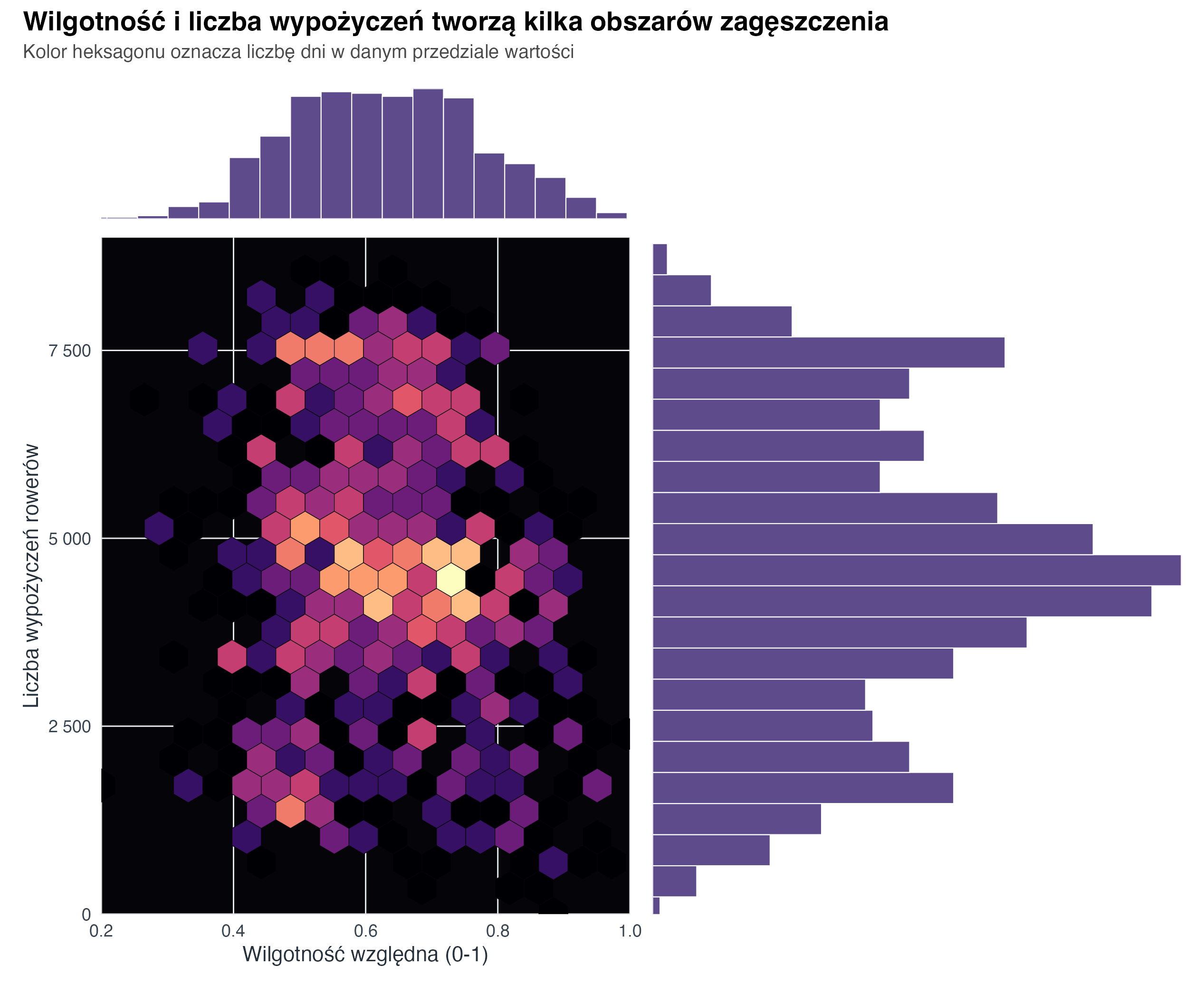
4.4 Heksagony i histogramy brzegowe

Gdy punktów jest dużo albo wartości nachodzą na siebie, pojedyncze kropki mogą ukrywać zagęszczenia. Wtedy dobrym wyborem jest wykres heksagonalny (hexbin plot): płaszczyzna jest dzielona na sześciokąty, a kolor pokazuje liczbę obserwacji w każdym z nich. Histogramy brzegowe dopowiadają, jak rozkłada się każda zmienna osobno.

bike_hex_limits <- list(
  x = c(0.2, 1),
  y = c(0, 9000)
)

bike_axis_theme <- theme(
  panel.grid = element_line(colour = "#2D2D35", linewidth = 0.25),
  panel.background = element_rect(fill = "#050509", colour = NA),
  plot.background = element_rect(fill = "white", colour = NA),
  axis.title = element_text(size = 11),
  axis.text = element_text(size = 9),
  plot.margin = margin(4, 6, 4, 6)
)

bike_margin_theme <- theme_void() +
  theme(plot.margin = margin(2, 6, 2, 6))

bike_hex <- bike_share |>
  ggplot(aes(x = hum, y = total_rentals)) +
  geom_hex(bins = 22, colour = "#050509", linewidth = 0.15, show.legend = FALSE) +
  scale_fill_viridis_c(option = "magma", trans = "sqrt") +
  coord_cartesian(xlim = bike_hex_limits$x, ylim = bike_hex_limits$y, expand = FALSE) +
  scale_x_continuous(labels = scales::label_number(accuracy = 0.1)) +
  scale_y_continuous(labels = scales::label_number(big.mark = " ")) +
  labs(
    x = "Wilgotność względna (0-1)",
    y = "Liczba wypożyczeń rowerów"
  ) +
  bike_axis_theme

bike_humidity_hist <- bike_share |>
  ggplot(aes(x = hum)) +
  geom_histogram(bins = 22, fill = "#5E4B8B", colour = "white", linewidth = 0.25) +
  coord_cartesian(xlim = bike_hex_limits$x, expand = FALSE) +
  bike_margin_theme

bike_rentals_hist <- bike_share |>
  ggplot(aes(x = total_rentals)) +
  geom_histogram(bins = 22, fill = "#5E4B8B", colour = "white", linewidth = 0.25) +
  coord_flip(xlim = bike_hex_limits$y, expand = FALSE) +
  bike_margin_theme

((bike_humidity_hist + plot_spacer()) /
  (bike_hex + bike_rentals_hist)) +
  plot_layout(widths = c(5.4, 1.05), heights = c(1, 5.2)) +
  plot_annotation(
    title = "Wilgotność i liczba wypożyczeń tworzą kilka obszarów zagęszczenia",
    subtitle = "Kolor heksagonu oznacza liczbę dni w danym przedziale wartości",
    theme = theme(
      plot.title = element_text(face = "bold", size = 14, margin = margin(b = 4)),
      plot.subtitle = element_text(size = 10, colour = "#4A4A4A", margin = margin(b = 8))
    )
  )

Rysunek 4.6: Wykres heksagonalny z histogramami brzegowymi dla wilgotności i liczby wypożyczeń rowerów.

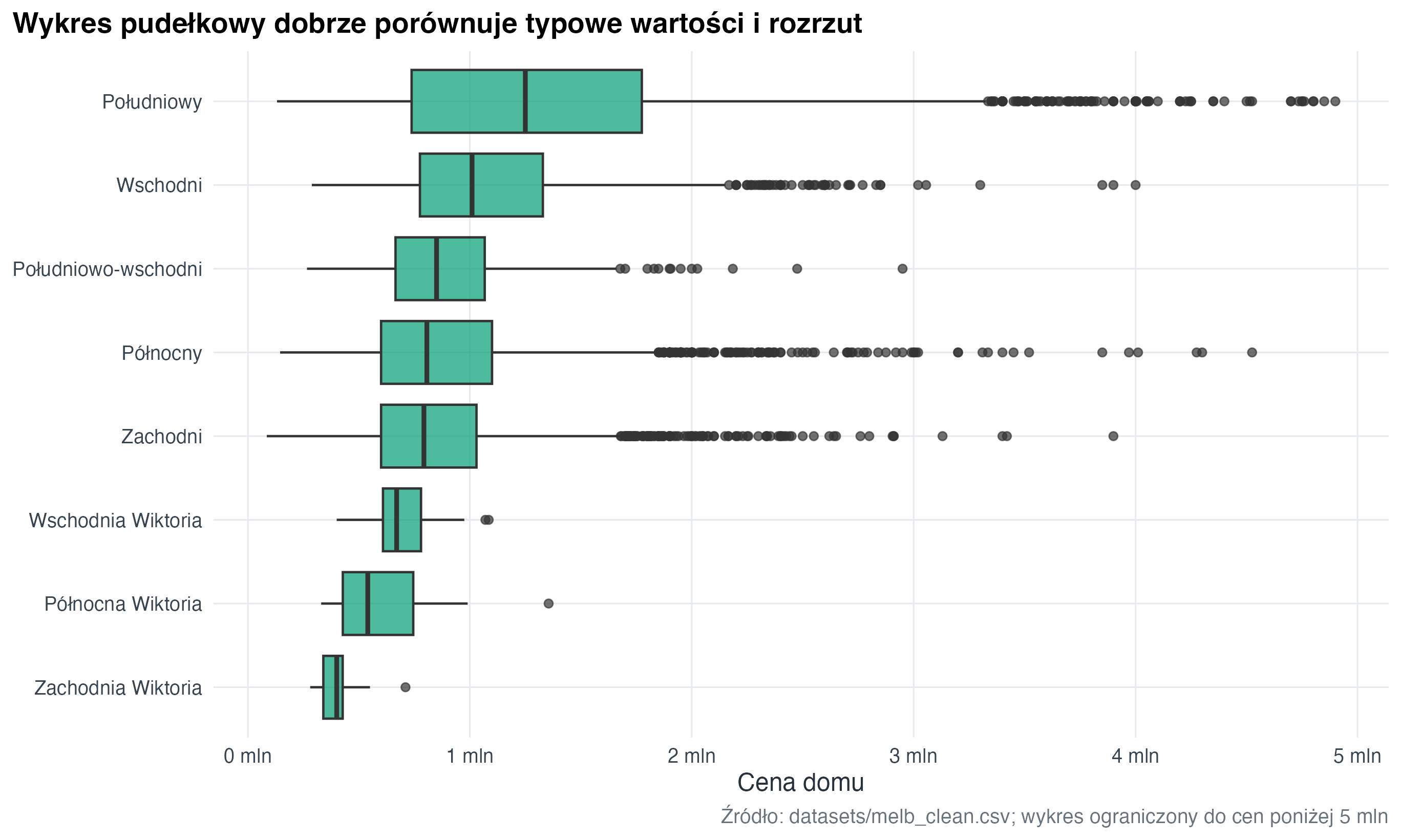
4.5 Wykres pudełkowy (boxplot) dla porównań

melb |>
  filter(!is.na(region), !is.na(price_m), price_m < 5) |>
  mutate(region = forcats::fct_reorder(region, price_m, .fun = median, na.rm = TRUE)) |>
  ggplot(aes(x = price_m, y = region)) +
  geom_boxplot(fill = "#009E73", alpha = 0.7, outlier_alpha = 0.25) +
  scale_x_continuous(labels = scales::label_number(suffix = " mln")) +
  labs(
    title = "Wykres pudełkowy dobrze porównuje typowe wartości i rozrzut",
    x = "Cena domu",
    y = NULL,
    caption = "Źródło: datasets/melb_clean.csv; wykres ograniczony do cen poniżej 5 mln"
  )

Rysunek 4.7: Ceny domów w Melbourne według regionu.

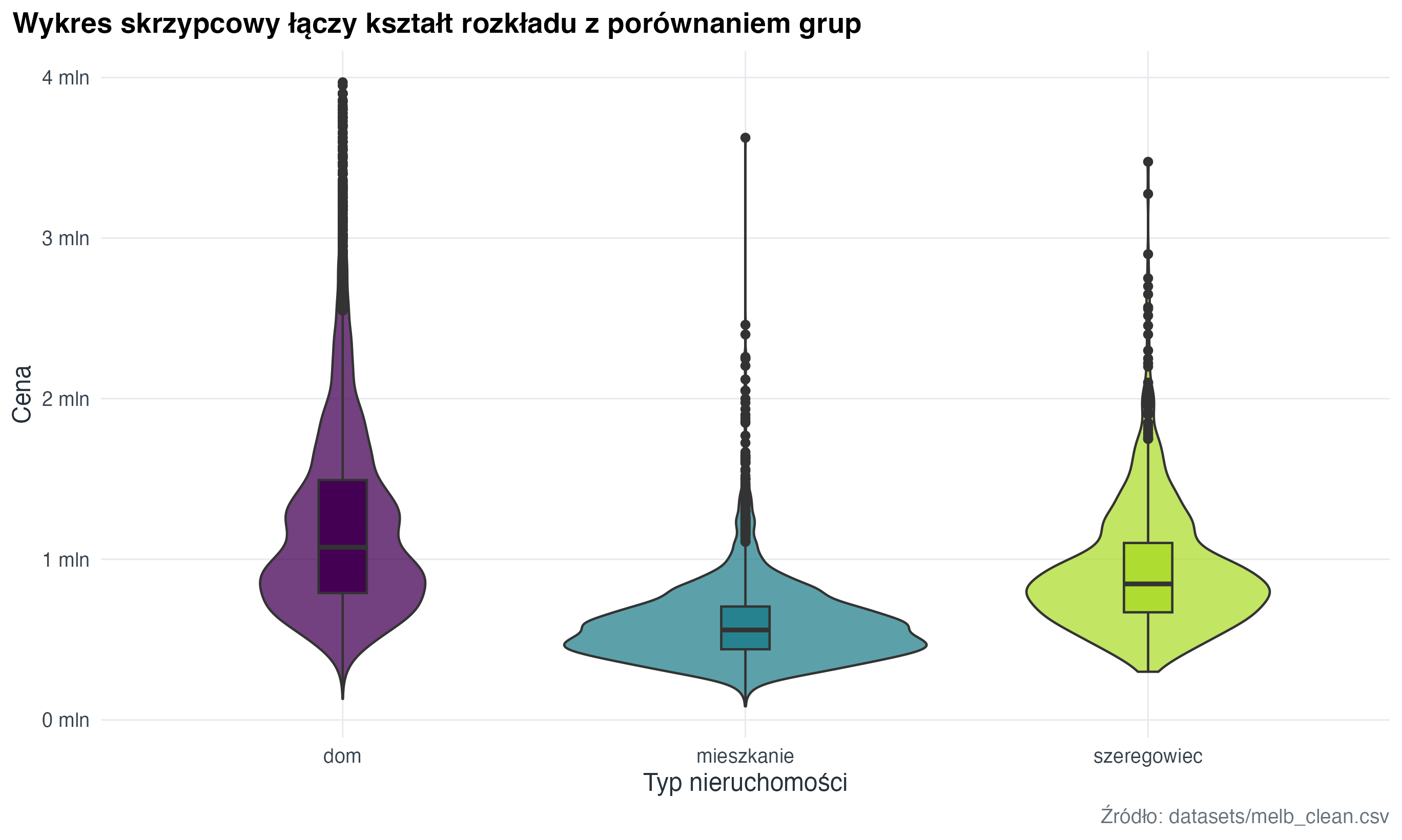
4.6 Wykres skrzypcowy (violin plot)

melb |>
  filter(!is.na(type), !is.na(price_m), price_m < 4) |>
  ggplot(aes(x = type, y = price_m, fill = type)) +
  geom_violin(trim = TRUE, alpha = 0.75, show.legend = FALSE) +
  geom_boxplot(width = 0.12, outlier_alpha = 0.2, show.legend = FALSE) +
  scale_fill_course_d() +
  scale_y_continuous(labels = scales::label_number(suffix = " mln")) +
  labs(
    title = "Wykres skrzypcowy łączy kształt rozkładu z porównaniem grup",
    x = "Typ nieruchomości",
    y = "Cena",
    caption = "Źródło: datasets/melb_clean.csv"
  )

Rysunek 4.8: Kształt rozkładu cen dla typów nieruchomości.

4.7 Zadanie

Dla fmr_1, fmr_2 i fmr_3 przygotuj trzy histogramy w jednym widoku. Podpowiedź: użyj pivot_longer() i podziel wynik na panele przez facet_wrap().