7  Małe wielokrotności

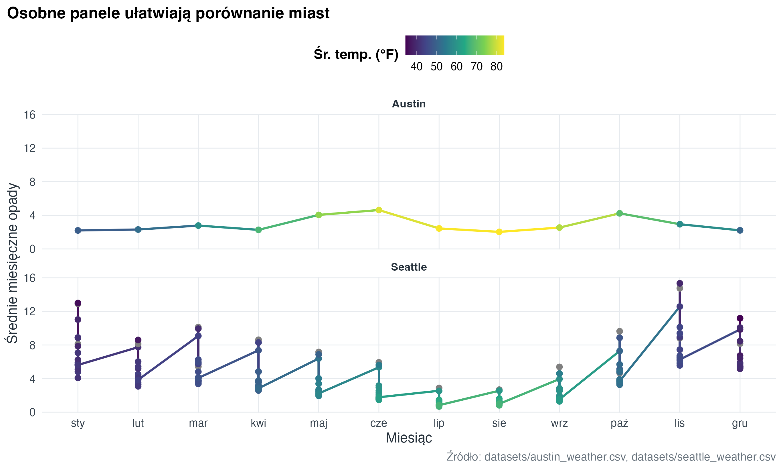
Małe wielokrotności (small multiples) są najlepsze wtedy, gdy chcemy porównać ten sam wzorzec w wielu grupach. Zamiast kodować wszystko kolorem, dajemy każdej grupie własny panel.

library(tidyverse)
library(here)
library(janitor)

source(here("R", "theme_course.R"))
theme_set(theme_course())

7.1 Pogoda w dwóch miastach

read_weather <- function(file, city) {
  month_labels <- c("sty", "lut", "mar", "kwi", "maj", "cze", "lip", "sie", "wrz", "paź", "lis", "gru")

  readr::read_csv(
    here("datasets", file),
    na = c("", "NA", "-7777"),
    show_col_types = FALSE
  ) |>
    janitor::clean_names() |>
    transmute(
      city = city,
      month_num = as.integer(date),
      month = factor(month_labels[month_num], levels = month_labels),
      precipitation = mly_prcp_normal,
      avg_temp = mly_tavg_normal
    )
}

weather <- bind_rows(
  read_weather("austin_weather.csv", "Austin"),
  read_weather("seattle_weather.csv", "Seattle")
)

weather |>
  ggplot(aes(x = month, y = precipitation, group = city, colour = avg_temp)) +
  geom_line(linewidth = 0.9) +
  geom_point(size = 2) +
  facet_wrap(vars(city), ncol = 1) +
  scale_colour_viridis_c(option = "D", name = "Śr. temp. (°F)") +
  labs(
    title = "Osobne panele ułatwiają porównanie miast",
    x = "Miesiąc",
    y = "Średnie miesięczne opady",
    caption = "Źródło: datasets/austin_weather.csv, datasets/seattle_weather.csv"
  )

Rysunek 7.1: Opady i temperatura w Austin oraz Seattle.

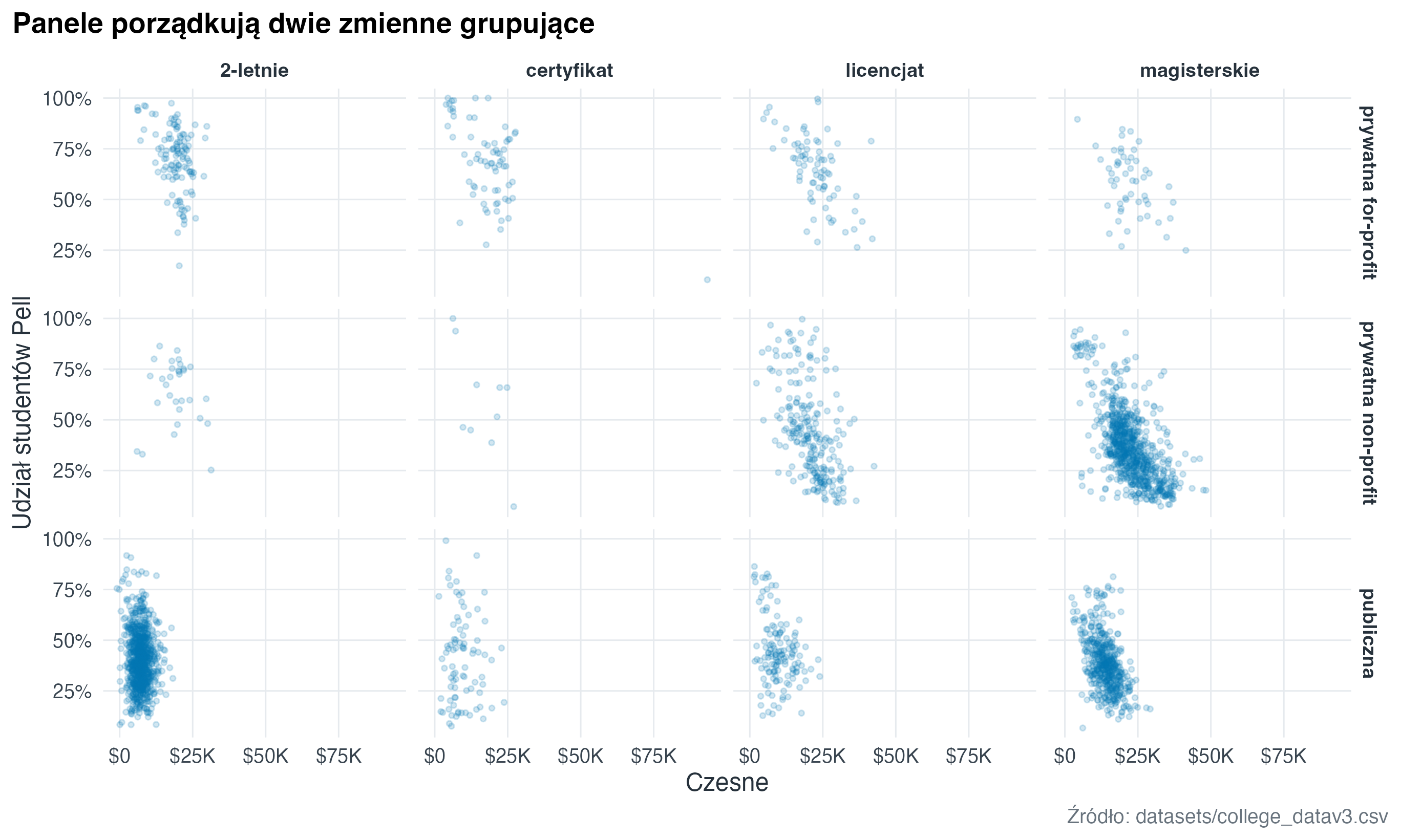
7.2 Podział na panele według dwóch zmiennych (facet grid)

college <- readr::read_csv(here("datasets", "college_datav3.csv"), show_col_types = FALSE) |>
  janitor::clean_names() |>
  filter(
    !is.na(tuition),
    !is.na(pctpell),
    !is.na(degree_type),
    !is.na(ownership),
    ug > 250
  ) |>
  mutate(
    ownership = recode(
      ownership,
      Public = "publiczna",
      `Private non-profit` = "prywatna non-profit",
      `Private for-profit` = "prywatna for-profit"
    ),
    degree_type = recode(
      degree_type,
      Graduate = "magisterskie",
      Associates = "2-letnie",
      Bachelors = "licencjat",
      Certificate = "certyfikat",
      `Non-degree` = "bez dyplomu"
    )
  )

college |>
  ggplot(aes(x = tuition, y = pctpell)) +
  geom_point(alpha = 0.18, colour = "#0072B2", size = 0.9) +
  facet_grid(ownership ~ degree_type) +
  scale_x_continuous(labels = scales::label_dollar(scale_cut = scales::cut_short_scale())) +
  scale_y_continuous(labels = scales::label_percent()) +
  labs(
    title = "Panele porządkują dwie zmienne grupujące",
    x = "Czesne",
    y = "Udział studentów Pell",
    caption = "Źródło: datasets/college_datav3.csv"
  )

Rysunek 7.2: Czesne i udział studentów Pell według typu uczelni.

7.3 Zadanie

Wykonaj wersję wykresu uczelni z facet_wrap(vars(degree_type)), czyli z jednym podziałem na panele. Która wersja lepiej odpowiada na pytanie o różnice między typami uczelni?